Evaluating a cheminformatics dataset - Part 1: An ML engineering and DevOps showcase

So far, my career path led me from analytical chemistry to data science, where I gained further experience in ML engineering, DevOps, and software engineering. In the first part of this showcase series I want to focus on the ML engineering and DevOps part of evaluating a cheminformatics dataset, where we will dive deeper into the following topics:

• Understanding the dataset/the problem
• Developing an extract, load, transform (ELT) workflow
• Train, validate, and test machine learning (ML) models
• Transferring the ELT workflow and ML processes into robust and scalable pipelines
• Explore real-world production scenarios

In the second part of this showcase series, which will be released later in a separate article, we will focus on the software engineering aspect. In general, we will follow a top-down approach when going through this showcase, meaning that we are creating a complete running workflow first, with a focus on the orchestration and selection of tools. Therefore, we will only see some high-level code snippets in this first part of my showcase series. In the second part (released as a separate article in future) we will dive deeper into the codebase and explore software engineering best practices like creating clean and maintainable code, following test-driven design principles and establishing a proper software lifecycle.

If you want to jump directly into the following first part of the showcase, you can go directly to Dataset and Problem.

Otherwise, I want to give a brief introduction how an analytical chemist finds their way into ML engineering, DevOps, and software engineering in the following preface.

Preface

While the path from data science (DS) to data engineering (DE), or software engineering (SWE) to DevOps sounds quite logical, one might ask, how analytical chemistry fits into this puzzle. But there is actually a common thread.

As an analytical chemist, you are working with analytical instruments, that generate analytical data of the samples that were measured. With modern instruments you are able to generate huge datasets, which detect even the tiniest amounts of a chemical compound in a mixture. Therefore, you are able to detect thousands of signals (so-called features) with only one measurement. In the early days of these analyses, when only a few features were present, a manual data evaluation was no problem. However, with ever-increasing datasets this is no longer feasible, which is why computational approaches became increasingly popular.

This leads an analytical chemist into the field of chemometrics, which is the field of gaining insights into (analytical) chemical datasets with the use of statistical-, bioinformatical-, or computational methods in general. While chemometrics is quite a narrow term for working with chemical datasets, it is basically a section of data science as a broader term. This is because we are evaluating and cleaning data, applying statistical/machine learning models on it, and eventually creating reports based on our insights and findings. This is the basic workflow for any dataset, and it doesn’t necessarily need to be a dataset with chemical information.

But how do we go from DS to DE, over DevOps to SWE? I started my chemometrics/DS journey already in academia and usually (or in my case, I don’t want to generalize here) you are starting with some scripts or Jupyter notebooks in R or Python. This totally works and yields (publishable) results. But when transitioning out of academia into the industry, you have some different rules. Of course, you need results, but you also need to consider things like maintainability, accessibility, interoperability, versioning, lifecycle management and so on and so forth. Then you realize, that a single script or Jupyter notebook flying around might not be the final solution.

This leads a data scientist into the field of SWE. Now you need to ensure that your data evaluation code follows clean-code principles, that is easy to read and maintain, not only by yourself but also by others. You also need to ensure that you follow a specific code architecture, that not only allows us to deal with your current data evaluation problem, but is also able to be modified in a way to deal with multiple problems in the future, without the necessity for a complete refactor every time a new problem/data evaluation comes up. Now, we are not thinking in scripts or notebooks anymore but in modules, libraries, and packages.

When following SWE best practices you naturally dive into the field of DevOps. You can have the best code in the world but to effectively use it, we also need to be aware of some DevOps principles like properly testing your code in automated ways, or performing systematic deployments of versioned packages to your users. So we not only need to deal with our code in a regulated manner, but also with the infrastructure.

And where is DE now located? In DS, we are figuring out, what the best statistical/machine learning models and data processing possibilities for our problem are, while using some DS languages like R or Python. In the best case we are following SWE principles. With DevOps, we are piping software and infrastructure together in a reproducible manner for productive environments. For smaller datasets or start-up environments, sophisticated DE principles aren’t absolutely necessary. But if datasets get bigger, coming in faster, and need to be processed in a reproducible and scalable way, then we arrived in the area of DE.

All of these disciplines work together and for every specialized task an own term exists. Like if you are more specialized on deploying ML models, you are more in the field of ML engineering. Or if you are more specialized on designing software products than building them, you are more in the field of software architecture than software engineering. But in practice, you are specialized in a thing but do also a bit of everything and the transitions are smooth.

But now let’s jump into the showcase starting with our dataset or “problem”.

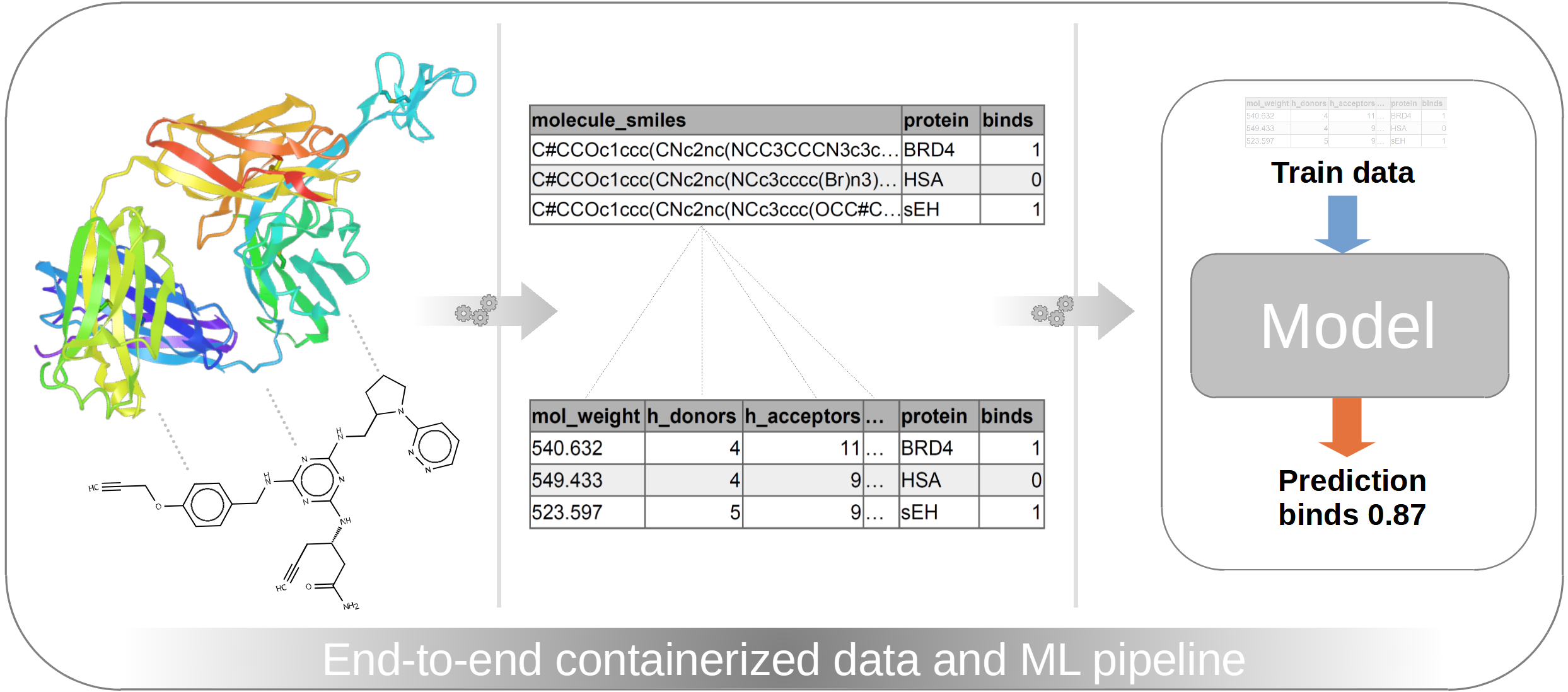
Dataset and problem

I didn’t want to use a hypothetical dummy dataset for this showcase but something that resembles a real-world problem. Also, it should be in the field of chemistry and be available to everyone. So I took a look at Kaggle first, since I am participating in some competitions there from time to time. There I found the NeurIPS 2024 - Predict New Medicines with BELKA competition.

In this challenge it shall be predicted if specific small-molecules bind to specific proteins. Given are the structural information of the small molecules, protein names, and the information if binding occurs or not.

And why did I exactly pick this challenge and not any chemistry related dataset on Kaggle or Hugging Face for instance? Oftentimes Kaggle challenges contain especially huge datasets, that put our skills to the test. So in order to even process the whole dataset of 300 million measurements, we are basically forced to use some advanced data/software/DevOps techniques. Furthermore, with such a challenge we are able to simulate the model deployment and inference in production by submitting results to the challenge.

But I don’t want to jump ahead. Let’s do that step by step. So we have now defined our dataset and our problem and in the next step we want to dive into the data.

Inspecting the data

After we downloaded all the challenge files mentioned above and unzip them, we have the following files:

• train.csv (52.7 GB)
• train.parquet (3.7 GB)
• test.csv (300 MB)
• test.parquet (30 MB)
• sample_submission.csv (23 MB)

As the sample names suggest, we have our train dataset, a test dataset and a sample submission file. For now, let’s focus just on the datasets. Each, the train- and the test dataset are available as csv and parquet file. Content-wise it doesn’t matter if you use the csv or parquet file. However, performance-wise there is a huge difference. It’s already obvious that parquet files are much smaller than csv files. But also due to their internal structure, they can be queried much faster. However, parquet files aren’t in a human-readable format compared to csv.

But since we are working with tools, that can handle parquet files, we can directly get rid of the csv files. Despite the sample submission file, of course

Now let’s check the content and shapes of train.parquet and test.parquet. I don’t go into any code at this point, and we just look at the data (Figure 1) to understand what we are dealing with.

In figure 1 we see the first lines of the train dataset. There are over 295 million rows and 7 columns. There is a unique id for every row and three SMILES code columns for the building blocks (buildingblock_smiles, SMILES is a computer-readable format for chemical structures). These three building blocks were used to synthesize the final small-molecule, as depicted by the molecule_smiles column. Then there is a protein_name column and a column that tells if the specific small-molecule per row binds to the specific protein or not.

The following overview of the test dataset looks nearly the same (Figure 2).

However, in figure 2 there are fewer rows (1.6 million) and one column is missing: the binds column. But that’s intentional, since the binds column is what we want to predict.

So to summarize the aim of this challenge: The aim is to predict if a specific small-molecule (depicted by their SMILES codes/chemical structure) binds to a specific protein (depicted by the protein name) or not.

Just based on looking at the data, we can already get some insights and ideas, how to proceed with the data.

Gaining first insights from the data

Since this showcase will focus on ML engineering and DevOps we won’t do much DS here. We will just get some basic insights and set up a plan, how to continue with the data to set up our pipelines and workflows.

So the first insights are basically, that we have 4 columns with SMILES codes but the molecule_smiles column is the most important, since these are the actual molecules that bind to the proteins.

If you look closer into the values of the molecule_smiles column you will see, that there is always a Dy in it. Usually, SMILES codes contain only Elements and how they are connected. However, there is no Dysprosium (element symbol Dy) in any of these molecules. In this specific dataset Dy just marks the position where the small-molecules were linked to the DNA.

Where does the DNA now come from? Basically, we don’t really need to care about it. We need to care about if the small-molecule binds to the protein. That the small-molecules are also linked to DNA is just due to the screening method, that was chosen by the authors.

So for us this means, we can get rid of the Dy in the molecule_smiles column since it’s not Dysprosium but just a marker for the DNA-link position.

But now, we basically only have the chemical structure of the small molecule, the name of the protein, and the information if the molecule binds to the protein or not. That’s not a lot of information to work with. So in the next steps we will develop the actual workflow starting with data cleaning and feature engineering.

Developing the workflow

As mentioned in the introduction we want to focus on ML engineering and DevOps techniques, which will really start in a later section. This section about developing the workflow including the subsections Data cleaning and feature engineering, Data transformations, and Model training, -validation, and -testing is, in this first part of the showcase, only covered on a high-level explaining our steps and goals, without diving deep into the code. The specific code developed and applied will later be discussed in part 2 of this showcase series in a separate article.

The development basically starts with extracting, transforming, and loading (ETL) or extracting, loading, and transforming (ELT) the data. At this point just a quick side note regarding the buzzwords ETL and ELT. While these concepts are often mentioned in data engineering context it’s not straight forward to map processes exactly to either ETL or ELT. Especially in data science/ML engineering steps are performed in between, that might not exactly belong to strict ETL/ELT definitions.

So my opinion about this is basically: We need to find and apply the right tools and technologies to efficiently pull our data and bring it in shape for our ML tasks. Is it now ELT or ETL or something in between? It doesn’t really matter as long as it works efficiently and you and your teammates are in agreement. I will therefore avoid ETL/ELT from now on and just explain what I am doing.

But after this sidenote let’s go back to the development of the workflow.

Data cleaning and feature engineering

With the chemical structures of the small molecules available, we can gather a lot further information, like the molecular weight, charges, sizes, and so on and so forth. For this we will use the Python package RDKit.

But before we pass SMILES codes to RDKit, we need to clean up the SMILES codes. Therefore, we simply need to get rid of Dy in the molecule_smiles column using polars. RDKit then returns molecular information that we are appending as new features (columns) to our dataset. For development, we start with just three different properties, which will later be expanded. These three properties are the molecular weight, the number of hydrogen bond donors, and the number of hydrogen bond acceptors as seen as new columns in figure 3.

In figure 3 we also see the cleaned molecule_smiles column with removed Dy. To test if the cleaning and feature engineering was successful we visually inspect the chemical formulas before, and after cleaning (Figure 4). For this we use the tool Ketcher, which can be directly used as a demo version in the browser.

As seen in figure 4, the DNA-link labelled with the Dy symbol was removed, which then also leads to the correct molecular weight of 540.63 g/mol. What also matches the molecular weight given in figure 3 (column “mw”). With this, the general plausibility of SMILES cleaning and molecular property calculation was confirmed. But we still can’t pass these data directly into our ML model for training. There are some final data transformation steps necessary that are explained in the next section.

Data transformations

As seen in figure 3 there are already new columns generated through feature engineering but there are still columns present, that are either not necessary or are in the wrong format. These are namely:

• All columns with SMILES codes
• The column storing the protein names

At first, we will remove everything, which is not necessary anymore and these are all columns storing SMILES codes. Why? Because the column molecule_smiles was already processed and is now represented with new numeric columns (mw, hbd, and hba). The other columns buildingblock1_smiles, buildingblock2_smiles, and buildingblock3_smiles are also just part of molecule_smiles and are therefore also not necessary anymore (since they are indirectly also represented by mw, hbd, and hba). So by removing all unnecessary columns first, we are left with this dataframe (Figure 5).

The column protein_name is very important, but it’s in the wrong format since it’s storing strings. For converting strings into numeric values we will use the OneHotEncoder from scikit-learn, which will create a new column for each unique element/protein in the protein_name column and assigns either 0 or 1. So in our case three new columns will replace the original column since there are three different proteins mentioned in the original column (Figure 6). We will also store the encoder as json file for later use.

Then we perform some final transformation steps. Since this is not a data science showcase I won’t go much into detail here and just list what we are doing then:

• Performing a simple 70/30 using scikit-learns train_test_split (gives us a train- and validation set)
• Train a StandardScaler from scikit learn on the train set, and store scaler as json file
• Apply the scaler on the validation set

The scaled train set and the scaled validation set are then used for model training and model validation.

Model training, validation, and testing

Since we want to focus on the ML engineering aspect in this showcase, we don’t spend much time on selecting and tuning the model architecture. We just use XGBoost since it usually performs quite well as a baseline and/or final model, and it uses the scikit-learn API, which makes the integration into our existing workflow quite easy. We will specifically use the XGBClassifier, since we want to predict if samples belong to one of the two classes: Either the molecule binds to the protein (1) or it doesn’t bind (0).

But to be exact, the aim of the Kaggle challenge is to predict the probability of a sample belonging to a class. But fortunately, the XGBClassifier class offers a predict_proba method, that yields the probability of belonging to each class.

So to make it short: We train the model on the train set and validate it on the validation set. Then fine-tuning of the model is performed to boost the metrics of our validation. Finally, the trained and fine-tuned model is stored as a json file and applied on the test set.

Quick recall, which set is what:

• The train set used for training the model is the 70 % portion of the train.parquet file
• The validation set used for validating the model is the 30 % portion of the train.parquet file
• The test set used for testing the model, or submitting the result to the challenge, respectively is the test.parquet file
• All subsets underwent the same cleaning-, feature engineering-, and data transformation processes

In conclusion, the complete workflow of data cleaning, feature engineering, data transforming like one-hot encoding and train-test splitting, as well as model training, -validating, and -testing is now complete. But during development of the complete workflow we only processed the first few rows of the dataset (usually around 10000). However, this needs to be done now for all ~300 million rows. While basic row/column transformations are handled by polars, so by Rust in the underlying architecture, these transformations are really fast. Also, the transformations handled by scikit-learn are really fast due to the usage of numpy, which relies on the C-language. But especially our RDKit operations are creating a bottleneck, since it’s mostly Python-based.

So our next challenge is to apply our complete workflow for all ~300 million rows in a robust and scalable pipeline.

Processing the full dataset in a robust and scalable pipeline

As mentioned in the prior section only around 10000 rows were processed to set up the workflow. There was no need to process all ~300 million rows since this would have slowed down the development drastically. But now, since the workflow is complete, we want to process all rows in order to pass the maximum of information (i.e. the full train set) into our machine learning model and to process the complete test set in order to submit a valid Kaggle challenge submission.

While this could basically all be done in a Jupyter notebook, since Kaggle doesn’t care “how” the submission file was created, we want to go a different route, because we want to focus on robustness and scalability to do justice to proper ML engineering- and DevOps principles.

But how are we achieving that? First, we need to consider what makes sense for our dataset and our available resources. Of course, we could rent high-end computational power on a cloud provider and set up a Kubernetes cluster to set up pipelines that are able to process terabytes of data in seconds, but especially in a company setting we should select the right tools to achieve the job in a cost-efficient way, but with scalability in mind.

So what are my considerations?

• The dataset is quite big, but it’s still manageable without the need of high-end cloud resources
• But we want to be open to process larger datasets in future on more potent machines (scalable)
• If we need to rerun the workflow in the future, everything should still work (robust)
• Instead of spreading the workflow execution across several technologies we start looking what GitLab provides since the repo is already there

So what exactly is the plan?

• Using GitLab CI/CD pipelines to run our workflow in defined stages
  • A personal computer utilized as a Gitlab runner utilizing Docker to provide more computational power in a cost-efficient way
  • Dockerized setup allows for further scalability
  • Controlling data processing, model training, and model inference version controlled via Git with additional UI features via GitLab
• Workflow is defined in a version controlled Python package
  • Provides robustness and maintainability
  • Utilization of GitLab CI/CD not only for processing, training etc., but also for code formatting, -linting and -testing

So now we have a plan and in the following we want to look closer at the individual components. Let’s start with looking at our CI/CD setup first and how to set up a GitLab runner.

Setting up a GitLab runner

While GitLab offers 400 min of runner runtime per month for free, this is just for a small runner with 2 vCPU cores, 8 GB RAM, and 30 GB storage. That runner is selected by default and is totally sufficient for simpler CI/CD tasks like linting or running (non-extensive) software tests. Of course, you can just use larger runners from GitLab, but that will become quite expensive quickly. Fortunately, it’s not that cumbersome to utilize your own computer as a GitLab runner.

Therefore, we want to use my personal computer as a GitLab runner, which has the following specifications:

• Intel Core i5 12600K CPU (10 cores, 16 threads)
• 80 GB DDR4 RAM
• Nvidia GeForce RTX 3080 GPU
• 1 TB NVME SSD

Especially RAM-size is a crucial factor, and we are equipped quite sufficiently with 80 GB. It’s a good starting point but barely not enough to process 300 million rows all at once. A fast NVME SSD is also crucial for data loading, -cleaning, and -processing, as well as a decent CPU. On the NVME part we are set but on the CPU part we could have done better, but we will now use what we have. The GPU is quite powerful for model training, however we are more focusing on the engineering part in this showcase and won’t, therefore, really utilize/need a powerful GPU.

On the software side only a few adjustments are necessary. Since GitLab runners are running Docker images we need to install Docker first. I am on a Windows machine, so I will install the Windows Docker Desktop client and, important, select WSL2 as the underlying architecture during the installation of Docker. You might need to install WSL2 first on your machine.

Then the Gitlab runner is installed and registered according to the official GitLab documentation. After the runner was installed we need to configure it. Therefore, we need a config.toml file in the same location as our gitlab-runner.exe, which looks as follows:

concurrent = 2
check_interval = 0
shutdown_timeout = 0

[session_server]
  session_timeout = 1800

[[runners]]
  name = "desktop-gpu-runner"
  url = "https://gitlab.com"
  id = <Some ID>
  token = <Some Token>
  token_obtained_at = <Some Date>
  token_expires_at = 0001-01-01T00:00:00Z
  executor = "docker"
  [runners.cache]
    MaxUploadedArchiveSize = 0
  [runners.docker]
    tls_verify = false
    image = "docker:edge-git"
    privileged = false
    disable_entrypoint_overwrite = false
    oom_kill_disable = false
    disable_cache = false
    volumes = ["/cache", "/var/run/docker.sock:/var/run/docker.sock", "/f/process_data/Leash:/mnt/data:rw", "/f/pip-cache:/root/.cache/pip:rw"]
    shm_size = 550000000000
    network_mtu = 0
    gpus = "all"

I want to highlight some lines since they are quite important:

volumes = ["/cache", "/var/run/docker.sock:/var/run/docker.sock", "/f/process_data/Leash:/mnt/data:rw", "/f/pip-cache:/root/.cache/pip:rw"]

These lines map some directories from the machine, where docker is running on, to the docker containers. The last two entries in this list map two directories from the f-drive to the container. One is a data directory and one is a cache directory.

In a company setting one would pull data e.g. from an S3 bucket or another cloud location. But since we are running our CI-jobs on a local runner, we can directly access the data from there. That’s much faster compared to downloading from a cloud location, and we don’t need to transfer a lot of data via the internet for every CI run. The same counts for our cache. Instead of downloading python packages each time we are starting a CI run, we download them once and cache them. In a company setting one would also store the cache in a cloud location, but we are also doing this on the local machine for the same reasons as for the data.

Another line is just gpus = "all" allowing us to use our GPUs also in the Container and finally name = "desktop-gpu-runner". This line assigns the tag, that is later used in the CI stages to target exactly this runner for specific CI jobs.

Defining the CI stages

Let’s look into the CI config, that orchestrates our workflow. In GitLab the CI is configured in a .gitlab-ci.yml file located in the root of the repository.

In the header of the .gitlab-ci.yml file we define some general rules first. So to use the latest Python version for instance or where to store the cache, some variables and what stages we have in total:

image: python:3.14-slim

cache:
  key:
    files:
      - pyproject.toml
      - requirements/*
  paths:
    - .cache/pip


variables:
  PIP_CACHE_DIR: "/root/.cache/pip"
  PYTHONUNBUFFERED: "1"  # logs/print statements will appear directly in the pipeline logs

stages:
  - check_code
  - prepare_train_data
  - train_model
  - prepare_test_data
  - test_model

After the header the actual stages are defined. The CI job linter and formatter are both part of the same stage check_code. That means that they can run in parallel since they are not really resource-intensive, especially due to the Rust-based formatter/linter ruff. Particular emphasis should be placed on the tags. Here we set our desktop-gpu-runner as the GitLab runner to use. If we don’t assign a tag, the default GitLab runners are used.

Side note: From now on you will read leash_bio quite often in the script section of the stages. This corresponds to the name of my Python package storing the scripts and modules of our workflow.

linter:
  stage: check_code
  tags:
    - desktop-gpu-runner
  before_script:
    - pip install -r requirements/linter.in
  script:
    - ruff check leash_bio

formatter:
  stage: check_code
  tags:
    - desktop-gpu-runner
  before_script:
    - pip install -r requirements/linter.in
  script:
    - ruff format --diff leash_bio

Now we come to the actual stages of our workflow. The stage prepare_train_data executes the script load_transform_data.py. In this script the tasks described in Data cleaning and feature engineering and Data transformations are executed. The result is batch-wise written to parquet files. This has two advantages:

• We are able to monitor the progress due to batch-wise processing
• If only subsequent stages/scripts are changed in the future, we don’t need to reprocess everything again since the parquet files act as checkpoints

Important line in this and the following stages: when: manual. With this the stages are only executed when actively selected. With this we are, e.g. able to only let the train_model stage run if we perform changes there and don’t need to let run prepare_train_data again if the stage already ran in the past and no changes were performed in this stage.

prepare_train_data:
  stage: prepare_train_data
  tags:
    - desktop-gpu-runner
  variables:
    DATA_TYPE: "train"
  before_script:
    - pip install --upgrade pip
    - pip install .
    # symlink to make the mounted data available for the python scripts
    - ln -s /mnt/data ./data
  script:
    - python "leash_bio/load_transform_data.py"
  when: manual

The train_model stage executes the script train_model.py where the XGBClassifier is trained on the train data as mentioned in Model training, validation, and testing.

train_model:
  stage: train_model
  tags:
    - desktop-gpu-runner
  before_script:
    - pip install --upgrade pip
    - pip install .
    # symlink to make the mounted data available for the python scripts
    - ln -s /mnt/data ./data
  script:
    - python "leash_bio/train_model.py"
  when: manual

Until now, only train data from train.parquet (see Inspecting the data) were processed. The trained model as well as the calibrated one-hot encoder and the standard scaler were exported as json files to be used in the following stages.

In the next stages we continue with the test.parquet file, were we perform the exact same data processing as on the train set. The only difference is, that we use the precalibrated one-hot encoder and standard scaler.

prepare_test_data:
  stage: prepare_test_data
  tags:
    - desktop-gpu-runner
  variables:
    DATA_TYPE: "test"
  before_script:
    - pip install --upgrade pip
    - pip install .
    # symlink to make the mounted data available for the python scripts
    - ln -s /mnt/data ./data
  script:
    - python "leash_bio/load_transform_data.py"
  when: manual

After the test data were processed the model inference is carried out on these data using the trained XGBClassifier as mentioned in Model training, validation, and testing.

In the end a submission csv file is produced in the same format as the kaggle challenge suggests by the sample submission (see Inspecting the data).

test_model:
  stage: test_model
  tags:
    - desktop-gpu-runner
  before_script:
    - pip install --upgrade pip
    - pip install .
    # symlink to make the mounted data available for the python scripts
    - ln -s /mnt/data ./data
  script:
    - python "leash_bio/test_model.py"
  when: manual

With this our workflow is now embedded into robust pipeline stages, since the .gitlab-ci.yml file is part of the version controlled repository. We also set the basis for scalability since currently we used the desktop-gpu-runner tag. Later we can just set up more potent machines, e.g. cloud resources, and just change the tag to target different machines for stage execution.

Executing the CI stages

Until now that all sounds a bit theoretical. How would that perform now in practice? What has one now to do if data shall be loaded, a model trained, and test results produced?

So let’s say our repository/Python package storing the workflow is fully equipped with a functional CI config (i.e. .gitlab-ci.yml file) as defined above. Then one just needs to commit to the repository and pipelines are triggered as seen in figure 7.

As you can see above in figure 7, only the formatter and linter from the check_code stage are automatically executed. That’s intentional since linting and formatting shall be carried out with each commit. And these jobs aren’t resource-intensive anyway. But all the following stages are halted (Figure 7 and 8) as defined by the manual tag in the CI config (see Defining the CI stages). By clicking on “run” on the individual stage it’s getting executed (Figure 8).

Since it’s the first execution of the workflow, we let all stages run (Figure 9). Don’t be misled by the run time of only 8:10 minutes. This was just a demonstration run not processing all rows.

Let’s recall what happened, after all stages were executed:

• Train data were processed and stored as parquet files, e.g. on an S3 bucket or in some other cloud location
• Calibrated encoders and scalers are stored as json files also in some cloud location
• A machine learning model is trained and also stored in some cloud location
• The model is used to perform inference on test data and results are exported to some cloud location

How can this now be utilized in production. Let’s look at some scenarios.

Production scenarios

The demonstrated workflow sounds interesting on paper but how would this now be applied in some real-world production scenarios?

Scenario A - New training data is available (rerun of all stages)

Usually, we don’t have a defined train dataset that never changes over the lifecycle of such a workflow. If we refer to our specific Kaggle competition dataset, that provides results of lab experiments (molecule binds to proteins or not), continuously new results might come in. So our train set will continuously be expanded. How would we treat that scenario in our workflow? So basically we will upload the new train.parquet file to our cloud location and run the stages again. Usually we would only add new measurements, so that we don’t need to reprocess the initial train dataset.

So in this scenario, we need to repeat every stage since the training data influences the complete workflow. But there are further scenarios where we might not need to rerun everything.

Scenario B - New ML model architecture (skipping stages)

Let’s say our data stays the same since the lab experiments were part of a finished project. But some time later a sophisticated new ML architecture is published, that we want to apply onto our data. In this case we will just commit the changes to the underlying train_model.py script in the train_model stage (see Defining the CI stages). Since all parquet files and encoders/scalers are still present in our cloud location, we just need to execute the model training and testing again and skip stages we don’t need (Figure 10).

Skipping stages that we don’t need saves a lot of time especially during development. However, if time and resources are available, I would still trigger a complete workflow run in the end after development, to be really sure that everything still works together.

Scenario C - Summary of further scenarios

So basically it boils down to the two scenarios “complete rerun” and “skipping stages”. So I will just summarize some further production examples and to which scenario they might belong.

• New test data available for inference -> skip all stages but the last test-model stage
• New data processing procedures shall be implemented -> complete rerun
• Software maintenance (dependency upgrades, refactoring etc.) -> complete rerun but with reduced datasets (see upcoming part 2 of this showcase)

Summary and outlook

In this first part of the showcase about the evaluation of a cheminformatics dataset with a focus on ML engineering and DevOps principles we set up a robust and scalable pipeline that processes our data and trains a machine learning model on it, that is later used to create predictions for a Kaggle challenge.

To set up and execute pipelines we used GitLab CI/CD. This was the perfect tool for our use case since we are already storing our workflow code as a repository there. So it just makes sense to directly use these resources instead of spinning up further external tools. Don’t get me wrong: There are fantastic tools out there, that can also be used for these tasks like Apache Airflow, Apache Spark, AWS SageMaker, or Databricks, and they make total sense in company settings where you have to deal with data that comes in high frequencies and with huge datasets in general.

But maybe we will also work on a project in the future using one of these tools. Also, what was currently not thoroughly discussed was the monitoring, especially of the ML model training with tools like MLFlow. I will implement that in future into this article, or in a separate one, but we will cover that for sure.

But for now: Thanks for reading and stay tuned for the second part of this showcase, which will be released soon.